Forecasting Volatility Using Machine Learning
Comparing traditional models to the LSTM model, for predicting the volatility of equities
“Only when the tide goes out do you discover who’s been swimming naked.”
Warren Buffett
Understanding the volatility of financial assets is important for several reasons:
Risk management: Volatility is a key measure of risk. Measures such as VaR (value at risk) depend on accurate future measures of volatility.
Asset allocation: Volatility is often a key input in portfolio construction and optimization. For example, for risk parity portfolios or mean-variance optimization.
Derivates pricing: The prices of derivative contracts, for example, options, are directly linked to expectations of future volatility of the underlying.
Market making: Forecasting bid / ask spreads is crucial to the market maker’s ability to maintain a liquid book. Spreads are influenced by volatility.
Given this importance, historically there has been an interest in forecasting future financial asset price volatility.
Traditional volatility forecasting models
Simple MA or EWMA
First, the simplest forecast of the volatility that one can think of is to use the average past volatility itself.
In this way, we can compute future volatility as simply the average of past, squared, price returns for an asset r(t). If we allow the weights to be w(t)=1/t then we have a simple average.
Alternatively, we could set w(t) such that they are exponentially declining further back in time so that we estimate volatility as an exponentially weighted moving average (EWMA).
We find they are mathematically quite sophisticated in their statistical formulation when switching to modern volatility models.1
ARCH model
Perhaps the most widely known, and applied, is the ARCH model by Robert Engle from 1982. The ARCH model, with parameter p, models the volatility as a function of past squared returns: 2
And where epsilon(t) is a standard normal distributed IID random variable.
So we can see how “volatility clustering” is captured by this model. Essentially if past returns have been larger in magnitude, the more we believe today’s volatility will be large. Therefore, volatility (or the squared returns — the return’s absolute magnitude) is persistent in time.
Given the wide success of ARCH, there have been innumerable variations to this basic model. The GARCH model, EGARCH, STARCH, IGARCH, TGARCH, CGARCH… the list goes on.
The basic improvement, however, came with the GARCH model in 1986 via Bollerslev, who modified the model above by adding lagged {sigma(t-1), sigma(t-2), … sigma(t-q)} terms to the right-hand side formula.
This allows the volatility forecast to be smoother, and it turns out the GARCH volatility is equivalent to an EWMA of past squared returns, but where the exponential weights are determined by statistical estimation, to maximize the fit of the GARCH model, not via an arbitrary choice.
The SV model
The SV or Stochastic Volatility model was an alternative to the ARCH model, published by Taylor in 1982. The main difference with the SV model is that it assumes volatility isn’t driven entirely by past returns, but rather there is a “hidden” factor h(t) driving volatility we cannot observe directly. The SV model is as follows:
Because this volatility is “hidden” it makes the model more statistically complex to estimate, and perhaps for this purpose alone, it never gained as much widespread use or popularity.3 That said the inherent flexibility provided by the hidden state of the model can lead to richer volatility dynamics.
ML Volatility Forecasting Models
Given this review of previous attempts at volatility forecasting, how can more modern machine learning (ML) based models contribute? Can they improve on the traditional models?
While there are a plethora of different models we could choose, given the historical precedent of building volatility models on time-series input data (in particular historical returns r(t)), we thought it would be interesting to try and build a model around the LSTM architecture, which was published by Hochreiter & Schmidhuber in 1997.
The LSTM (or GRU) model
The LSTM (or “long short-term memory” model) has been used successfully in time-series forecasting tasks, within several fields, including speech recognition, electricity grid power load, industrial goods demand, and other natural phenomena.
The LSTM is particularly interesting in this case, since similarly to the SV model above, at its core it has a “hidden” state variable that drives the dynamics of the predictions.
However, the dynamics of the hidden state are designed to encompass both a “short-term” and “long-term” memory of the past values of the input variables. That is, at least in theory, the model should “remember” both recent episodes of volatility as well as those from the distant past.
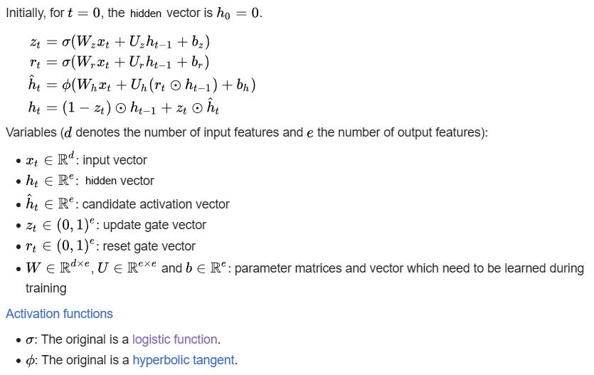
For our purposes we’ll use a simpler version of the LSTM, called the GRU model, which has shown similar performance in most tests of time-series forecasting, but reduces the complexity of the model significantly. The mathematical formulation of the GRU model is as follows: 4
Essentially the GRU is a hidden state model where what the hidden state is allowed to remember is modulated by the z(t) and r(t) “gates.” z(t) affects the long-term memory of the process, and r(t) affects the short-term memory.
Note that r(t) above is not asset price returns as was the case previously. Rather, price returns enter into the model as the input vector:
This formulation is again similar to the SV model in that it assumes that squared returns (i.e. volatility) are log-Normally distributed. That is, taking logs of squared returns leads to x(t) which is roughly Normally distributed.
At any given time, we then predict future volatility as:
Typically we let f be a linear mapping function, but it need not be so. We can also allow for f to take as input a history of {h(t), h(t-1), …, h(t-s)} hidden states. The hidden state vector h(t) itself is allowed to be multidimensional, even though the input is of dimension 1.5
Empirical Comparison
For this empirical comparison, we will forecast daily volatility for AAPL stock, 1-day into the future. Of course, different, longer-term, forecast periods could be implemented if need be.
We fit the ARCH, GARCH, and GRU models to daily AAPL closing price stock returns, as described above.
For the ARCH and GARCH models, we allow for hyperparameters p=5, and p=q=5, respectively. For the GRU, the hyperparameterization can be complex so we simply search the parameter space for something that results in useful predictions.
Everything is out-of-sample (i.e. we train on a train set, and then forecast on a previously unused test set, using an expanding train window as time progresses), and the only hyperparameter search we do is for the GRU. The models in both cases are retrained every 42 trading days (2 months roughly).
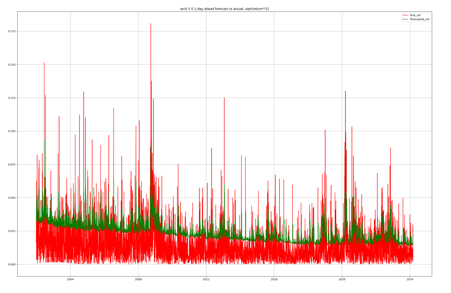
ARCH(5) results
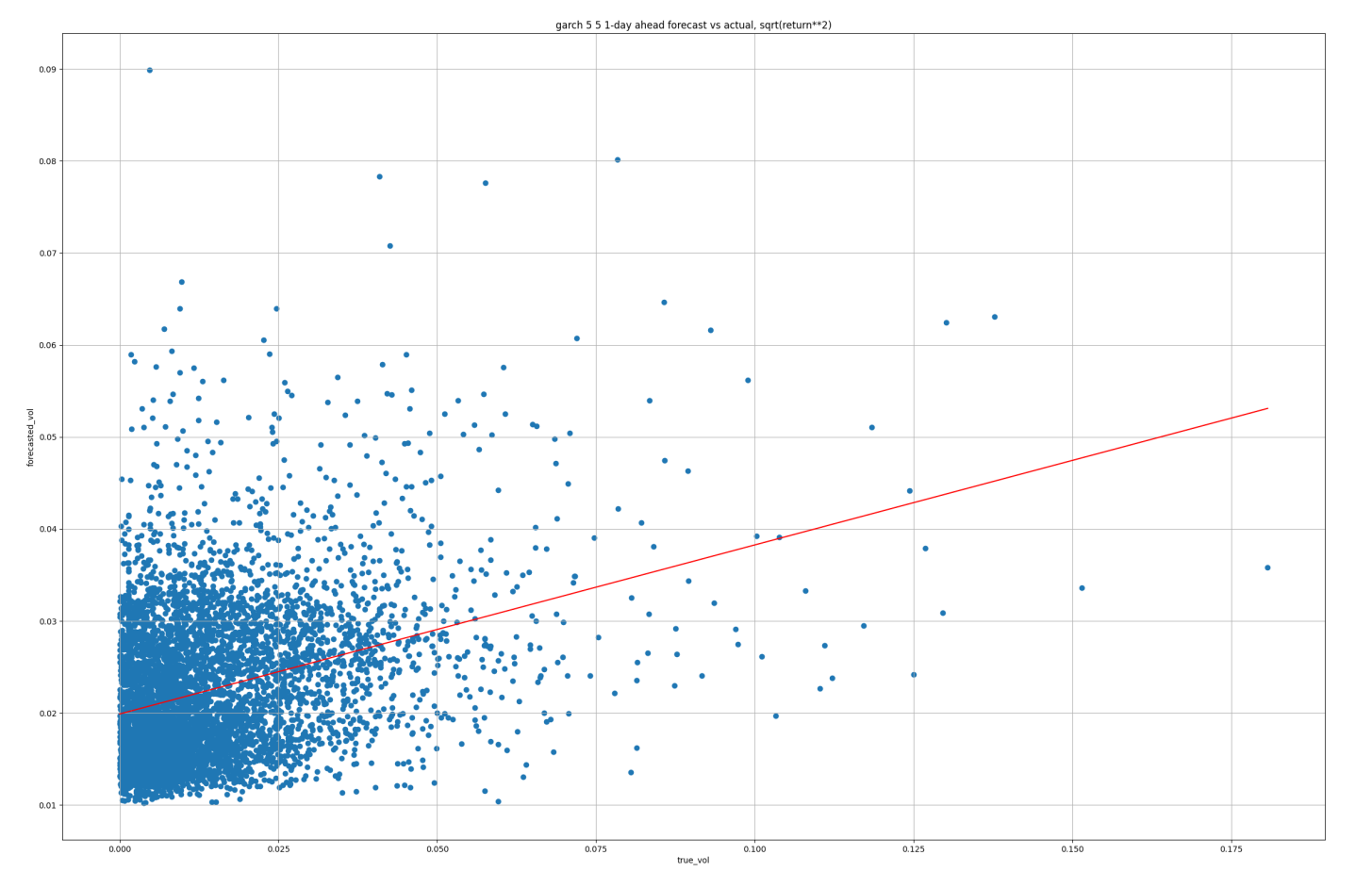
GARCH(5,5) results
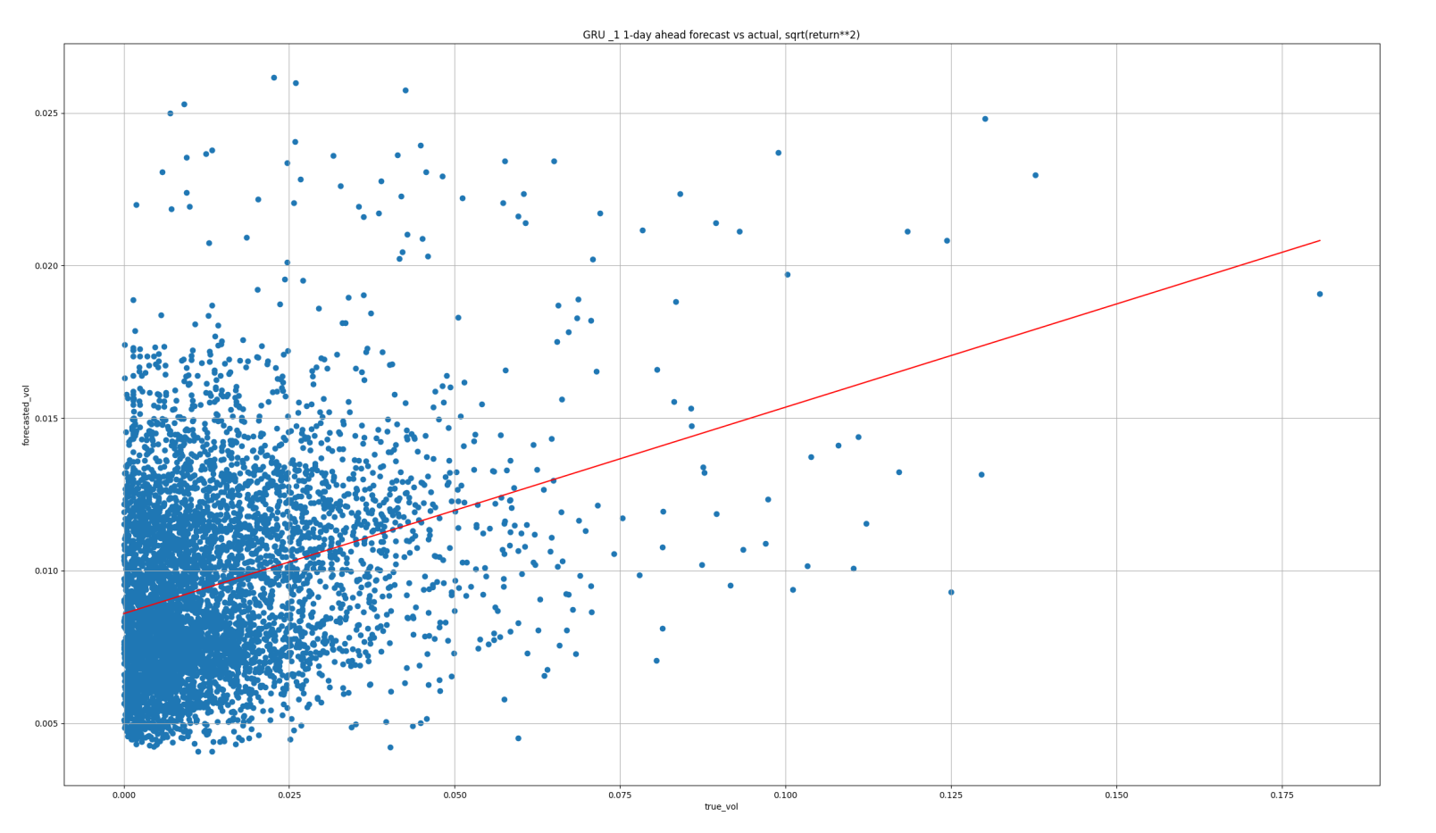
GRU results
Results comparison
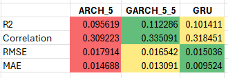
We compare the results across three metrics:
Root mean squared error (RMSE)
This metric will put more weight on large outliers in predictive errors
Mean average error (MAE)
This metric cares more about the average error and doesn’t over-weight outliers
R-squared (R2)
This is the measure of variance explained by the model versus that left unexplained by the model. The larger the value the better the fit.
In this case, the R2 is based on the OLS regression line plotted on each scatter in red. Since the model is linear, sqrt(R2) is the correlation between the forecast and true values.
The results suggest that the GRU is the superior model. In particular about MAE, where the reduction is quite significant. The reason is obvious if we look at the time-series plots of the predictions above. In both the ARCH & GARCH examples, the forecasts are much too large on average.
However, in all cases, the scatters reveal that much of the low-volatility periods are overestimated; we can see this by the fact that the red OLS line slopes are typically less than 1.
Moreover, there is likely some nonlinearity not being captured here. Potentially the GRU could be improved by implementing the f output mapping function as nonlinear.
Conclusion
In summary, we’ve discussed the following:
The significance of understanding the volatility of financial assets, highlighting its importance in risk management, asset allocation, derivatives pricing, and market making.
We then reviewed traditional volatility forecasting models such as the simple moving average (MA), exponentially weighted moving average (EWMA), ARCH model, and stochastic volatility (SV) model.
Next, we introduced modern machine learning (ML) based models, particularly focusing on the long short-term memory (LSTM) and gated recurrent unit (GRU) models, as potential improvements over traditional methods.
Finally, an empirical comparison was conducted between ARCH, GARCH, and GRU models in forecasting daily volatility for AAPL stock, with metrics including root mean squared error (RMSE), mean average error (MAE), and R-squared.
The results suggested that the GRU model outperforms ARCH and GARCH models, particularly in terms of MAE, although there are indications that further improvements could be made by implementing nonlinear output mapping functions in the GRU model.
This follows in the spirit of other mathematically influenced pricing models, such as the Black-Scholes model for the price of a European put/call option, which itself involves the volatility of the underlying as an input parameter. See Black-Scholes Wikipedia.
Where for simplicity we use demeaned returns to avoid the use of the mu term.
The hidden h(t) can be estimated via a linear Gaussian state-space model, albeit inefficiently, since nu(t) is not Gaussian, and the model must be log-linearized to form a linear observation equation.
The model performs significantly better when the hidden state is allowed to be multidimensional.


