Understanding Security Sensitivity to Good and Bad Times Through Mixture Models
We explore how to leverage Gaussian Mixture Models (GMM) to model regime dependent betas
While investors have often suspected that a security’s price sensitivity to the overall market varies across time, and can change dramatically during periods of market turmoil, it’s not entirely clear how to measure this phenomenon.
One approach taken is to divide up our historical sample of security prices, and subjectively judge which periods we believe represent the regimes of interest (e.g. periods of low vs high market volatility, periods of market drawdowns, etc).
While this approach can be useful, its main drawback is how it relies on our subjective assessments of what represented historically a “good” or “bad” period for the market.
In this article, we’ll instead turn to an alternative approach that relies on statistically modelling the processes underlying the security in question (and the market as a whole) as Gaussian mixtures.
Gaussian Mixture Models
The Gaussian in the name refers to the academic name applied to the so-called Bell-curve, or “Normal,” distribution we’re all familiar with.
A Gaussian mixture is therefore a mixture of Bell-curve distributions.
It turns out that mixing Bell-curve distributions has the desirable property that it can well represent the distribution of a security (or the market’s) price returns, that aren’t themselves actually Normally distributed.
Moreover, using such a mixture can help us identify when a security’s return was generated during either a “good” or “bad” regime.1
Essentially we want to use the Gaussian mixture model (herein GMM) to discover the security’s return distributions for both the “good” and “bad” states of the market.
We then want to determine the sensitivity of the security’s price returns to the market as a whole during these “good” and “bad” states, in comparing them.
This sensitivity is usually measured as Beta, and we will maintain that convention here as well. Therefore, the GMM model facilitates comparison of the security’s measured Beta during the “good” and “bad” states automatically.
Finally, we can use the GMM model to determine which state the security’s price was in, historically.
In this sense, the GMM can be considered a “regime model.”
Example Setup - GMM on Barrick Gold
For this particular example, we will use the market’s current, and lagged returns, as the inputs that determine the regime state at any time ‘t’.2
Our proxy for the market will be the SPDR S&P500 ETF (ticker: SPY).
The target security for the model is chosen as Barrick Gold (ticker: GOLD).
Why Barrick Gold?
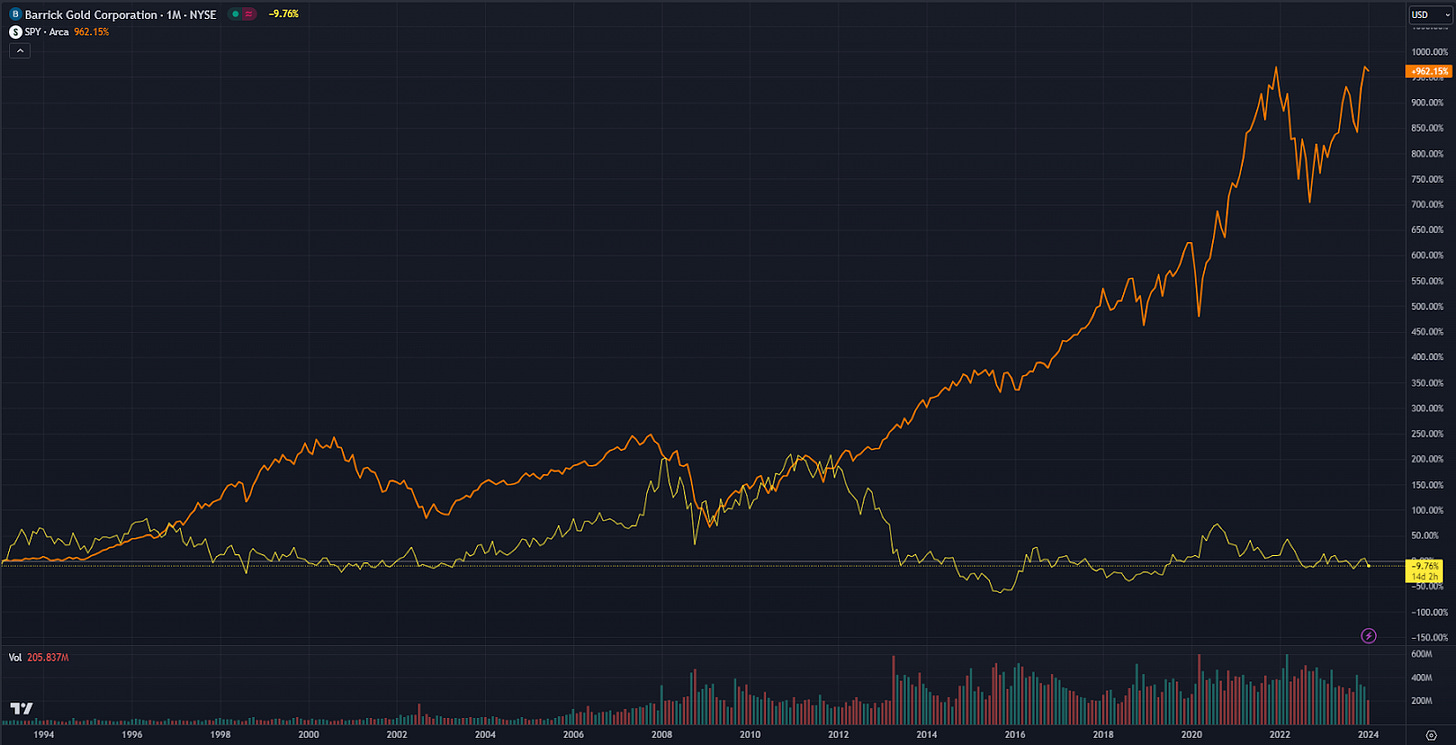
Barrick Gold is chosen as an example here, given the oft-cited expectation that its Beta is roughly zero.
The story goes, that Barrick Gold, being a gold mining company, shouldn’t in principle be affected by what happens in the equity markets.
We will show that during periods of market crisis, the Beta on Barrick Gold stock can change dramatically.
Model details
We leave most of the technical details on how to estimate the GMM model in the appendix of Tashman & Frey 2009 and only focus on the details necessary for intuition on how the model works.3
Essentially, model estimation amounts to choosing the model parameters so that they maximize the probability that, given the observed returns data for GOLD and SPY, the GMM model fits the data.
Finally, note, we apply the model to monthly security returns in order to capture longer term phenomena. The data runs from 1993 until today, and involves 371 data points.
The two individual states
Since the GMM involves two states, and each state represents a Gaussian distribution on Barrick Gold’s returns, in either the “good” or “bad” state, we can understand these two Gaussian distributions as representing essentially two CAPM style regression models:
Here r_i,t is Barrick Gold’s monthly return at time ‘t’, and r_m,t is SPY’s monthly return.
Therefore, for each state i={0,1} (i.e. good and bad states) α_i is the expected return to Barrick Gold if SPY’s return equals 0 during that period, and β_i is the Beta of Barrick Gold to SPY.
e_i,t is a residual that represents variation not explained by the model. The standard deviation (i.e. volatility) of this residual represents the volatility of Barrick Gold not explained by the market. We denote this volatility of e_i,t as σ_i. Finally, note that since the model is Gaussian, so is e_i,t.
Thus there are two sets of parameters for each regression: α_i, β_i, and σ_i, so six parameters so far in total.
The State Determination Model
Now, how does the GMM model determine which regime state the market is in at any given time?
As discussed above, for simplicity, we use current and lagged values of SPY to inform this regime state decision (but we could augment this with additional variables if we wanted to).
For this example, we allow for the contemporaneous SPY return (i.e. r_m,t) and one lagged value (i.e. r_m,t-1).
That is, SPY’s current return, and last month’s return, are used to estimate the current time ‘t’ regime state, as being either i={0,1} (as well as all historical state values).
Let’s now denote the parameters associated with current and lagged SPY as γ_1 and γ_2.
In this model, the effect of SPY returns on the regime state is determined by a Logistic function4, similar to how a logistic regression works.
For simplicity, you can think of the following function defining the probability we are in state 0, at time ‘t’: 5
The logistic function 𝑓(﹒) is such that as ɡ_t increases, the probability increases we are in state 0.
In this sense, you can think of ɡ_t as a weighted average of the current and last period return of SPY, where the γ values are the weights. If the γ values are both positive, then larger current and past SPY returns mean a higher probability of state 0.
So with the addition of γ_1 and γ_2, we now have 8 model parameters that need to be estimated.
Estimation results
We estimate the model on monthly Barrick Gold returns and find the following results (where alpha and sigma values have been annualized):
Looking at the results, we interpret that the “bad” state is state 0, and the “good” state is state 1.
In the good state 1, we find:
An annualized return to Barrick gold of 10.91% when SPY is zero.
An annualized idiosyncratic volatility of 29.5%.
The Beta between Barrick Gold and SPY is 0.004.
However, in the bad state 0, we find:
An annualized return to Barrick gold of 6.12% when SPY is zero.
An annualized idiosyncratic volatility of 46.9%.
The Beta between Barrick Gold and SPY is 0.621.
Therefore, during periods of market turmoil, Barrick Gold’s Beta increases from near zero to 0.621.
One explanation for this behavior is investor crowding. During crisis periods investors crowd into Barrick gold stock, thus increasing its directional movement with the market.
Note, that such dramatic differences in Betas between regime states do not appear to be common.
A similar application of the GMM model to monthly returns for both IBM and GE stock didn’t reveal large differences in Betas between the “good” and “bad” states.
Another notable feature of the estimated parameters is that both gamma values are negative.
This means that the larger (i.e. more positive) the current and past SPY returns, the more likely we are in state 1, the good state. This implies that states, at least in this context, tend to persist and so the state itself exhibits momentum. 6
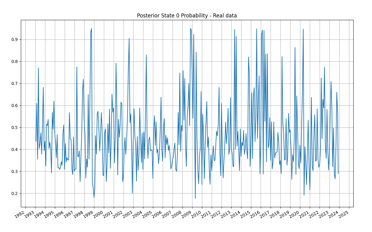
What follows is a monthly time series plot of the probability that we are in state 0 (the bad state) conditional on observing Barrick Gold returns: 7
We can see in this plot that the probability we are in a bad state tends to increase in periods we would expect, such as late 2007 and 2008, 2015 and 2016, and during the Covid crash of Feb 2020.
Moreover, on average, the probabilities tend to suggest we experience the good state more than the bad, and there is a positive skew in the distribution towards the bad state.
Finally, a useful application of the GMM model is for hedging. If we know that Betas differ across regimes, and we have the means to estimate, dynamically, which regime state we are currently in, we can adapt our hedge ratios appropriately to compensate.
Conclusion
In conclusion, we demonstrated how a Gaussian mixture model can be used to differentiate between historical regime states, and how one application for this type of regime analysis is to calculate differing security Betas between states. Moreover, such a model could be used for hedging.
The model isn’t limited to analysing security Betas, however, and given the flexibility of the model, other applications exist. For example, the model could be used to estimate return prediction models where the parameters of the models depend on regime states.
Finally, the regime states themselves need not be informed only by current and past market data. For example, economic indicators, or macro series, can easily be introduced into the model, to inform the regime state as well.
The model in this article borrows heavily from the article by Tashman & Frey entitled “Modeling risk in arbitrage strategies using finite mixtures.” The article was published in the journal “Quantitative Finance”, vol 9, issue 5, in 2009. The co-author Robert Frey was a managing director at Renaissance Technologies from 1992 to 2004. Thanks to Brandon Koepke for passing it along.
That said, this need not be so. Alternatively, we could use other variables, beyond the market’s current and past returns, to determine whether the market is in a good or bad state. For example, we could use economic indicators, the level of the VIX, the credit spread, or any other variable you can think of that as an investor you believe would affect the state of the market and its relationship to the security in question.
See footnote 1 above.
Also known as the Sigmoid function.
For the technically inclined, this is the prior distribution of state probabilities, before we observe any Barrick returns. The posterior distribution (i.e. the probability of being in each state, conditional on observing a Barrick Gold return) is a bit more complicated. See Tashman & Frey 2009 for details.
This isn’t necessarily going to be true in general. It isn’t hard to imagine that if we defined the model on daily or weekly data, there could be a reversal effect, where bad states follow good and vice versa.
i.e. the posterior distribution p(i={0,1}|r_t), where r_t is Barrick Gold’s return at time ‘t’.


